Machine learning (ML) is a subset of artificial intelligence (AI) that focuses on building systems that learn from data. It allows machines to improve at tasks with experience, using algorithms to analyse data, learn from it, and make predictions or decisions.
AI, on the other hand, is a broader field aiming to create machines capable of performing tasks that typically require human intelligence. This includes reasoning, perception, and understanding language. AI encompasses not only machine learning but also other approaches that do not require learning from data, such as rule-based systems.
Instead of being explicitly programmed to perform a task, ML systems improve their performance on a task over time with experience.
In summary, the predictive or classification model is created and is then tested in real-time. Based on its performance in real-time, it’s continually updated to maintain and improve its performance. It continues to ‘learn’ over time.
In the notes for this week we identified three types of machine learning models:
Supervised learning models, where we give the model data with explicit input and output variables. Examples of this approach would include discriminant analysis.
Unsupervised learning models, where we give the model data but don’t define any associations or relationships. It’s left to the model to ‘discover’ these. Examples of this approach would include cluster analysis.
Reinforcement learning models, where an agent learns to make decisions by interacting with an environment to achieve a goal. The agent learns from experiences, using trial and error, to perform actions that maximise cumulative rewards over time.
We’ll review examples of each of these models in the following sections.
71.2 Supervised learning
Theory
Supervised learning involves training a machine learning model on a labeled dataset, where the correct answer is provided, and the model learns to make predictions based on that data.
The model’s predictions are then compared to actual outcomes, or those of a testing dataset, to adjust the model accordingly. This type of learning is called “supervised” because an algorithm learning from the training dataset can be thought of as having a teacher supervising the learning process.
Regression: Demonstration
Linear regression is a simple example of supervised learning. As we covered earlier in the module, regression involves exploring the relative influence of different independent variables (IVs) on a dependent variable (DV).
In the following example I’m going to use the lm() function in R to predict the likelihood of basketball players winning season-ending awards.
The dataset includes player statistics such as points per game, assists, rebounds, etc.
I’ll prepare the data, create training and test sets, fit the linear model, and interpret the results.
# create synthetic datasetlibrary(tidyverse)# Set the seed for reproducibilityset.seed(123)player_stats <-tibble(player_id =1:100, # idaward =sample(c("MVP", "NoAward"), 100, replace =TRUE, prob =c(0.1, 0.9)),points_per_game =rnorm(100, mean =20, sd =5), # Normally distributed pointsassists =rnorm(100, mean =5, sd =2),rebounds =rnorm(100, mean =7, sd =3))# Create a dependent variable 'performance_score' that's a linear combination of the IVsplayer_stats <- player_stats %>%mutate(performance_score =50+2* points_per_game +3* assists +4* rebounds +rnorm(100, mean =0, sd =5))## create model# Fit regression modelmodel <-lm(performance_score ~ points_per_game + assists + rebounds, data = player_stats)# Summarise modelsummary(model)
Call:
lm(formula = performance_score ~ points_per_game + assists +
    rebounds, data = player_stats)

Residuals:
     Min       1Q   Median       3Q      Max
-12.6695  -2.7941   0.2623   2.7056  13.1528

Coefficients:
                Estimate Std. Error t value Pr(>|t|)
(Intercept)      53.9222     2.9601   18.22   <2e-16 ***
points_per_game   1.7899     0.1077   16.63   <2e-16 ***
assists           3.0966     0.2782   11.13   <2e-16 ***
rebounds          3.9169     0.1742   22.49   <2e-16 ***
---
Signif. codes:  0 '***' 0.001 '**' 0.01 '*' 0.05 '.' 0.1 ' ' 1

Residual standard error: 5.147 on 96 degrees of freedom
Multiple R-squared:  0.9031,    Adjusted R-squared:  0.9001
F-statistic: 298.3 on 3 and 96 DF,  p-value: < 2.2e-16
rm(model)
We didn’t go into much detail earlier in the module regarding the role of regression coefficients (the ‘estimates’) but they are important in the context of machine learning.
In the example above:
The coefficient of points_per_game is close to 2, indicating that for each additional point per game, the performance score increases by approximately 2 units, holding all else constant.
The coefficient of assists is just over 3, indicating that each additional assist is associated with a 3 unit increase in performance_score, holding all else constant.
The coefficient of rebounds is close to 4, showing that each additional rebound is associated with a 4 unit increase in performance_score, holding other factors constant.
So, these coefficients provide a quantifiable measure of the relationship between each independent variable and the dependent variable, reflecting the strength and direction (positive in this case) of these relationships.
You can also see that the adjusted R-squared is 0.90, suggesting that around 90% of the variability in the DV is explained by our IVs. This is a ‘good’ model.
Our model has therefore ‘learned’ how to predict future events. In the next game, if we know the points per game, the assists and the rebounds, we can use it to predict (with expected 90% accuracy) what the performance score is likely to be.
Of course, real life doesn’t always work like that. Bear that mind when getting excited about predictive modelling…
There is a problem with this approach, which we’ve covered before. It runs the regression on the entire dataset, and we now need to wait for ‘new’ data to check how effective the model performs in real life. This is called ‘overfitting’; we’ve created a model that is really good based only on the data we gave it.
As you know, one approach to this issue is to divide the data into training and testing datasets. We can create our model on the training data, and then see how it performs when given new, unseen data (the testing data).
# Load the necessary librarylibrary(caret)
Loading required package: lattice
Attaching package: 'caret'
The following object is masked from 'package:purrr':

    lift
# Split data into training and testing setsset.seed(123) # for reproducibilitytrainIndex <-createDataPartition(player_stats$performance_score, p = .8, list =FALSE, times =1)trainData <- player_stats[trainIndex, ]testData <- player_stats[-trainIndex, ]# Fit linear regression model on training datamodel <-lm(performance_score ~ points_per_game + assists + rebounds, data = trainData)# Summarise modelsummary(model)
Call:
lm(formula = performance_score ~ points_per_game + assists +
    rebounds, data = trainData)

Residuals:
     Min       1Q   Median       3Q      Max
-10.3405  -2.7734   0.2039   2.3772  12.8836

Coefficients:
                Estimate Std. Error t value Pr(>|t|)
(Intercept)      53.9569     2.9783   18.12   <2e-16 ***
points_per_game   1.7867     0.1120   15.96   <2e-16 ***
assists           3.1673     0.2870   11.04   <2e-16 ***
rebounds          3.9175     0.1738   22.53   <2e-16 ***
---
Signif. codes:  0 '***' 0.001 '**' 0.01 '*' 0.05 '.' 0.1 ' ' 1

Residual standard error: 4.791 on 76 degrees of freedom
Multiple R-squared:  0.9239,    Adjusted R-squared:  0.9209
F-statistic: 307.6 on 3 and 76 DF,  p-value: < 2.2e-16
# Predict on testing datapredictions <-predict(model, newdata = testData)# Evaluate model performancemse <-mean((predictions - testData$performance_score)^2)print(mse)
In this example, we divide our data into 80% training, and 20% testing. The MSE (40.56) tells us how well the model performed when presented with the unseen (testing) data.
Lower values of MSE mean better model performance. In this case, we have nothing to compare it with (and with a simple model like this, it’s unlikely we could create alternative models).
Using linear regression, predict the number of wins for a basketball team in a season using player statistics with linear regression.
When you’ve done a linear regression, replicate the process above where we created training and testing datasets, and inspect the MSE for this model.
show solution for linear regression
# Fit the linear regression modelmodel <-lm(wins ~ points_scored + points_allowed + total_rebounds + average_age + efficiency, data = team_stats)# Model Summarysummary(model)
Call:
lm(formula = wins ~ points_scored + points_allowed + total_rebounds +
    average_age + efficiency, data = team_stats)

Residuals:
    Min      1Q  Median      3Q     Max
-5.3440 -2.1355  0.0129  1.6548  5.5806

Coefficients:
                Estimate Std. Error t value Pr(>|t|)
(Intercept)     50.63560   33.46943   1.513   0.1434
points_scored    0.67836    0.28810   2.355   0.0271 *
points_allowed  -0.30343    0.31812  -0.954   0.3497
total_rebounds   0.74264    0.12201   6.087 2.75e-06 ***
average_age      0.03447    0.17818   0.193   0.8482
efficiency     -21.19079   27.73981  -0.764   0.4524
---
Signif. codes:  0 '***' 0.001 '**' 0.01 '*' 0.05 '.' 0.1 ' ' 1

Residual standard error: 3.022 on 24 degrees of freedom
Multiple R-squared:  0.8552,    Adjusted R-squared:  0.825
F-statistic: 28.35 on 5 and 24 DF,  p-value: 2.486e-09
show solution for linear regression
rm(model)
Code
# Load the necessary librarylibrary(caret)# Split the data into training and testing setsset.seed(123) trainIndex <-createDataPartition(team_stats$wins, p = .8, list =FALSE, times =1)trainData <- team_stats[trainIndex, ]testData <- team_stats[-trainIndex, ]# Fit linear regression model on the training datamodel <-lm(wins ~ points_scored + points_allowed + total_rebounds + average_age + efficiency, data = team_stats)summary(model)
Call:
lm(formula = wins ~ points_scored + points_allowed + total_rebounds +
    average_age + efficiency, data = team_stats)

Residuals:
    Min      1Q  Median      3Q     Max
-5.3440 -2.1355  0.0129  1.6548  5.5806

Coefficients:
                Estimate Std. Error t value Pr(>|t|)
(Intercept)     50.63560   33.46943   1.513   0.1434
points_scored    0.67836    0.28810   2.355   0.0271 *
points_allowed  -0.30343    0.31812  -0.954   0.3497
total_rebounds   0.74264    0.12201   6.087 2.75e-06 ***
average_age      0.03447    0.17818   0.193   0.8482
efficiency     -21.19079   27.73981  -0.764   0.4524
---
Signif. codes:  0 '***' 0.001 '**' 0.01 '*' 0.05 '.' 0.1 ' ' 1

Residual standard error: 3.022 on 24 degrees of freedom
Multiple R-squared:  0.8552,    Adjusted R-squared:  0.825
F-statistic: 28.35 on 5 and 24 DF,  p-value: 2.486e-09
‘Unsupervised learning’ is another type of machine learning algorithm used to draw inferences from datasets that contain input data, but without labeled responses. The most common unsupervised learning method is cluster analysis, which organises data into clusters based on similarity.
Unlike supervised learning, unsupervised learning algorithms are not provided with the correct results during training; they must find try to find structure within the input data on their own.
K-means Cluster Analysis: Demonstration
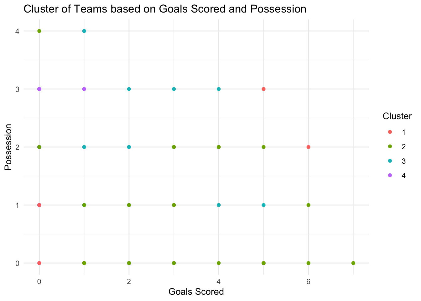
To demonstrate this, I’ll create a k-means cluster analysis that attempts to group football teams based on some of their playing statistics.
# Load librarylibrary(stats)## Create dataset# Num teamsnum_teams <-100# Initialise vectorsgoals_scored <-c()goals_conceded <-c()possession <-c()# Generate four distinct clusters# Cluster 1goals_scored <-c(goals_scored, rpois(num_teams /4, lambda =0.8))goals_conceded <-c(goals_conceded, rpois(num_teams /4, lambda =2))possession <-c(possession, runif(num_teams /4, min =45, max =50))# Cluster 2goals_scored <-c(goals_scored, rpois(num_teams /4, lambda =2))goals_conceded <-c(goals_conceded, rpois(num_teams /4, lambda =0.8))possession <-c(possession, runif(num_teams /4, min =55, max =60))# Cluster 3goals_scored <-c(goals_scored, rpois(num_teams /4, lambda =1.5))goals_conceded <-c(goals_conceded, rpois(num_teams /4, lambda =1.5))possession <-c(possession, runif(num_teams /4, min =50, max =55))# Cluster 4goals_scored <-c(goals_scored, rpois(num_teams /4, lambda =3))goals_conceded <-c(goals_conceded, rpois(num_teams /4, lambda =1))possession <-c(possession, runif(num_teams /4, min =40, max =45))# Combine into data framefootball_data <-data.frame(goals_scored, goals_conceded, possession)# Select relevant columns for clustering selected_columns <- football_data[, c("goals_scored", "goals_conceded", "possession")]# Perform k-means clusteringset.seed(123)clusters <-kmeans(selected_columns, centers =4) # Choose number of clusters# Attach cluster results to datafootball_data$cluster <- clusters$cluster# Examine clustershead(football_data)
library(ggplot2)ggplot(football_data, aes(x = goals_scored, y = goals_conceded, color =as.factor(cluster))) +geom_point() +labs(title ="Cluster of Teams based on Goals Scored and Possession",x ="Goals Scored",y ="Possession",color ="Cluster") +theme_minimal()
Hierarchical Cluster Analysis: Demonstration
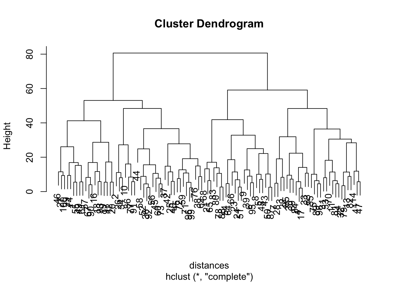
The second type of cluster analysis we introduced earlier in the module was hierarchical cluster analysis (HCA).
In this example, my objective is use HCA to identify distinct groups of tennis players based on their playing style.
# Load librarylibrary(stats)# Define the number of playersnum_players <-100# Generate synthetic dataserve_accuracy <-runif(num_players, 50, 90) # Serve accuracy between 50% to 90%return_points_won <-runif(num_players, 20, 70) # Return points won between 20% to 70%breakpoints_saved <-runif(num_players, 10, 80) # Breakpoints saved between 10% to 80%# Create a data frametennis_data <-data.frame(serve_accuracy, return_points_won, breakpoints_saved)##____________________# Select relevant columns for clusteringselected_columns <- tennis_data[, c("serve_accuracy", "return_points_won", "breakpoints_saved")]# Perform hierarchical clusteringdistances <-dist(selected_columns) # Calculate distances between playershc <-hclust(distances) # Perform hierarchical clustering# Plot the dendrogramplot(hc)
So, at this surface level, remember that k-means and hierarchical cluster analysis are both types of unsupervised learning models. They seek to find some ‘meaning’ in the data without us explicitly telling them where that meaning might lie.
71.4 Reinforcement learning
Theory
Reinforcement learning (RL) is a third type of machine learning. In this approach, an agent learns to make decisions by interacting with an environment.
The agent seeks to maximise some notion of cumulative reward over time through trial and error, learning from its successes and failures.
In reinforcement learning, the agent is not told which actions to take, but instead must discover which actions yield the most reward by trying them.
This process involves observing the current state of the environment, selecting and performing actions, and receiving rewards or penalties in return.
The goal is to create a policy. The policy is a strategy for choosing actions based on the current state that maximises the total future reward.
The key components of these RL systems are:
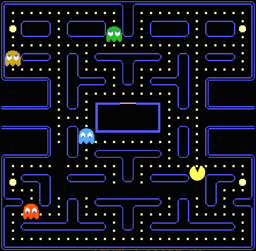
Agent: The learner or decision-maker. Think of it like pac-man.
Environment: The system with which the agent interacts. Think of it like the pac-man maze, and the various characters.
State: A representation of the current situation of the agent within the environment. What is pac-man’s situation right now?
Action: All the possible moves that the agent can take. Where can pac-man go right now?
Reward: An immediate return given to the agent for its actions, guiding it on what is ‘good’ or ‘bad’. Where would a better or worse place be for pac-man to go? Allocate rewards to the ‘better’ options.
Policy: A strategy that the agent employs to determine its actions based on the current state. Based on this analysis, create a general strategy for pac-man to follow.
Value function: This estimates the expected cumulative future rewards from each state, helping the agent predict long-term benefits.
Q-value or action-value function: This predicts the expected cumulative future rewards of taking a specific action in a given state.
Reinforcement learning algorithms can be classified into three main categories. We won’t go into detail here but they are:
Value-Based: The agent uses a value function to select actions without requiring a policy. For example, Q-learning is a value-based method that learns the value of action-state pairs.
Policy-Based: The agent learns a policy that specifies the best action to take without using a value function. An example is the REINFORCE algorithm, where the policy is directly optimized.
Model-Based: The agent builds a model of the environment’s dynamics and uses it for planning. This approach requires a model of the environment to predict future states and rewards.
The learning process in RL is iterative and based on updating the values of states or actions to better estimate the expected future rewards.
As noted, one common algorithm is Q-learning, where the agent updates the Q-values (estimates of future rewards for actions in states) using the Bellman equation, gradually improving its policy.
Demonstration
Introduction
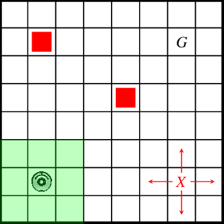
In this example of reinforcement learning we’ll use a simple grid world environment where an agent learns to navigate to a goal state.
In a ‘grid world’ environment, an agent learns to navigate through a grid to reach a goal state. The grid represents a space consisting of cells, each corresponding to a state.
The agent can move in different directions (e.g., up, down, left, right) and its objective is to find the optimal path to the goal while possibly avoiding obstacles or penalties.
In this environment, the agent receives rewards or punishments after each action, guiding its learning process. The reward structure typically includes positive rewards for reaching the goal, negative rewards (penalties) for hitting obstacles or undesirable states, and sometimes small negative rewards for each move to encourage efficiency.
The agent learns a policy - a mapping from states to actions - that maximises its cumulative future rewards. This is often achieved through methods like Q-learning or value iteration, where the agent iteratively updates its knowledge about the value of taking certain actions in specific states.
Preparation - define parameters
In this example, I’m not using any specific reinforcement learning package; instead, we’ll code a basic version of the Q-learning algorithm from scratch.
# load packagerm(list=ls())library(hash)
First, several key parameters for the Q-learning algorithm are initialised:
alpha: the learning rate, determining how much new information overrides old information.
gamma: the discount factor, balancing the importance of immediate and future rewards.
epsilon: the exploration rate, dictating how often the agent should try random actions as opposed to known best actions.
num_episodes: the number of episodes to run the training for.
# Initialise parametersalpha <-0.1# Learning rategamma <-0.9# Discount factorepsilon <-0.1# Exploration ratenum_episodes <-1000# Number of episodes for training
Initialise Q-table
Next, we initialise a Q-table using a ‘hash table’ in R, setting up the underlying structure for Q-learning:
Initialise Hash Table: Q <- hash() creates a new hash table1 and assigns it to the variable Q. A hash table is a data structure that efficiently stores key-value pairs.
Nested Loops: There are two nested for loops. The outer loop iterates over states (for (state in 1:4)), and the inner loop iterates over actions (for (action in 1:2)). In this context, there are 4 states (1 to 4) and 2 actions (1 and 2).
Populate Q-table: Inside the inner loop, the .set function is called: .set(Q, paste(state, action, sep="-"), 0). This function populates the Q-table with initial Q-values.
Specifically, it creates a key by concatenating the current state and action (e.g., “1-1”, “1-2”, “2-1”, etc.) using the paste function with a separator -. ItiInitializes the Q-value for each state-action pair to 0. This is a common initialisation strategy, starting with a neutral assessment of each action’s value in each state.
By the end of this code snippet, the Q-table Q contains all state-action pairs as keys, each initialised with a Q-value of 0, setting the stage for the learning process where these values will be iteratively updated based on the agent’s experiences.
Next, we define the environment for a simple reinforcement learning scenario, including the rules for state transitions and reward assignments based on actions taken by the agent:
Environment States:
There are 4 states labeled 1 through 4. State 1 is the starting point, states 2 and 3 are intermediate or “neutral” states, and state 4 is the goal.
Actions:
Two possible actions are defined: 1 (move forward) and 2 (move backward). In this context, moving backward from state 1 has no effect, since it’s the starting point
get_next_state Function:
This function calculates the next state given the current state and the action taken. If the action is 1 (move forward), it increases the state by 1, capped at state 4 (the goal). This ensures the agent doesn’t move beyond the goal state.
If the action is 2 (move backward), it decreases the state by 1, with a minimum limit of state 1. This prevents the agent from moving backward past the starting state. The min and max functions are used to enforce these upper and lower bounds, respectively.
get_reward Function:
This function determines the immediate reward received after moving to a new state. A reward of 1 is given if the next state is state 4 (the goal), signifying the agent has successfully reached the goal. A reward of 0 is given for all other transitions, indicating no immediate reward for moving to states 1, 2, or 3.
Together, these components simulate an environment where an agent learns to navigate from a starting point to a goal. The agent is rewarded for reaching the goal and uses the get_next_state and get_reward functions to understand the consequences of its actions, thereby learning to navigate the environment effectively.
# Define environment# States are: 1 = Start, 2 = Neutral, 3 = Neutral, 4 = Goal# Actions are: 1 = move forward, 2 = move backward (in this simple example, backward movement has no effect in state 1)get_next_state <-function(current_state, action) {if (action ==1) {return(min(current_state +1, 4)) } else {return(max(current_state -1, 1)) }}get_reward <-function(current_state, action, next_state) {if (next_state ==4) {return(1) # Reward for reaching the goal } else {return(0) # No reward for other transitions }}
Implement the algorithm
Finally, the following code implements a basic version of the Q-learning algorithm.
Here’s a concise description of its function:
Initialise the Learning Episode: The algorithm runs through a specified number of learning episodes (num_episodes), which are individual sequences of agent-environment interactions aiming to reach a goal.
Set Initial State: Each episode begins with the agent in the starting state (state 1), and the goal is to navigate to the goal state (state 4).
Action Selection (Exploration vs. Exploitation):
Exploration: With a probability (epsilon), the agent randomly selects an action (explore) to discover new strategies.
Exploitation: Otherwise, the agent chooses the action with the highest expected future reward based on current knowledge (exploit), comparing the Q-values of moving forward or backward from the current state.
Perform Action and Observe Outcome: The agent performs the selected action, transitions to the next state, and receives a reward. The transition and reward depend on the current state, the action taken, and the environment’s rules.
Q-value Update (Learning): The algorithm updates the Q-value, which is an estimate of the total future rewards the agent can expect by taking a given action in the current state. This update is based on the observed reward and the maximum Q-value of the next state, adjusted by the learning rate (alpha) and discount factor (gamma).
Loop Until Goal State: Steps 3 to 5 repeat until the agent reaches the goal state (state 4), concluding the episode.
Repeat for Additional Episodes: The entire process repeats for the specified number of episodes, with the agent gradually improving its strategy (policy) to maximise rewards through learning from the environment.
So, this code trains an agent to navigate a simple environment by learning from its experiences, optimising its decisions to achieve a goal efficiently.
# Implement Q-learningfor (episode in1:num_episodes) { current_state <-1# Start at the beginning of the environmentwhile (current_state !=4) { # Continue until goal state is reached# Select actionif (runif(1) < epsilon) { action <-sample(1:2, 1) # Explore } else {# Exploit: choose the best action based on current Q-values forward_value <- Q[[paste(current_state, 1, sep="-")]] backward_value <- Q[[paste(current_state, 2, sep="-")]]if (forward_value >= backward_value) { action <-1 } else { action <-2 } }# Take action and observe outcome next_state <-get_next_state(current_state, action) reward <-get_reward(current_state, action, next_state)# Q-learning update old_value <- Q[[paste(current_state, action, sep="-")]] next_max <-max(Q[[paste(next_state, 1, sep="-")]], Q[[paste(next_state, 2, sep="-")]]) new_value <- (1- alpha) * old_value + alpha * (reward + gamma * next_max).set(Q, paste(current_state, action, sep="-"), new_value) current_state <- next_state }}
Report
Now, we can print the Q-values. These Q-values represent the learned evaluations of how good it is to take a certain action in a given state, in terms of expected future rewards.
Here’s what the command reports:
Learned Q-values: The output will show the Q-values for each state-action pair in the environment. These values are the agent’s learned estimations of the expected cumulative future rewards for taking an action in a specific state.
State-Action Pairs: Each entry in the displayed Q-table corresponds to a specific state-action pair. For example, the Q-value associated with state 1 and action 2 would be the agent’s estimate of the expected reward for taking action 2 in state 1.
Policy Guidance: Indirectly, these Q-values provide insight into the policy the agent has learned. A higher Q-value for a specific state-action pair suggests that the action is more desirable in that state.
By examining these Q-values, we can understand the strategy or policy that the agent has learned through its experience, indicating which actions it considers best in each state based on the rewards it expects to receive.
When the agent is in state 1 and takes action 1, the expected return is 0.81.
1-2 : 0.728
In state 1, if the agent takes action 2, the expected return is approximately 0.728.
2-1 : 0.9
From state 2, taking action 1 yields the highest expected return so far, 0.9.
2-2 : 0.728
In state 2, action 2 has an expected return of about 0.726.
3-1 : 1
This indicates that when the agent is in state 3 and takes action 1, it achieves the maximum possible return of 1. This could indicate reaching the goal or receiving a maximum reward in this state-action scenario.
3-2 : 0.802
In state 3, taking action 2 results in an expected return of approximately 0.801.
4-1 : 0
For state 4, taking action 1 gives a return of 0. This could suggest that action 1 in state 4 is not beneficial or possibly that it leads to a terminal state with no further rewards.
4-2 : 0
Similarly, action 2 in state 4 also results in a return of 0, indicating no expected reward from this state-action pair, which might be another indication of a terminal or non-rewarding state.
Remember: the Q-values help in determining the optimal policy. For each state, the action with the highest Q-value would be chosen. For example, in state 2, the agent would (according to the policy) choose action 1 since 0.9 is greater than 0.73. The goal in reinforcement learning is typically to maximise these Q-values through learning, thereby maximising the expected cumulative reward.
In Q-learning, a hash table is a data structure used to store and retrieve the Q-values associated with different state-action pairs.↩︎